STEP 2: Velocity model estimation
Seismic velocity estimation (also referred to as seismic velocity model building, or even tomography) is usually the most challenging step of the seismic imaging workflow, and the focus of my dissertation work. It is the process of estimating the speed at which the waves travel through the ground, referred to as a seismic velocity model. The wave speed highly depends on the type of rocks in which sound propagates, and typically ranges from 1.5 km/s for water to 7 km/s for volcanic rocks within the subsurface (compared to 0.3 km/s in the air).
Full waveform inversion (FWI): the industry standard
In the last decade, one particular tomogaphic algorithm referred to as full waveform inversion (FWI) has become the industry standard for velocity model building (largely due to the increased computational power) and many case studies have shown its potential at recovering accurate and high-resolution solutions. This algorithm requires two inputs: seismic data, and an approximate initial guess of the solution (referred to as the initial model), and is then applied in an iterative manner as follows:
- Using the initial velocity model, a seismic survey (similar to the one acquired on the field) is simulated on a computer
- The simulated seismic data is compared to the field data
- If the two datasets are not "similar" enough (according to a pre-defined metric), this lack of similarity (also called error, misfit or residual) is translated into an update of the velocity model, gradually improving its accuracy
- This iterative procedure is performed until the simulated seismic data becomes "similar" enough to the field data. And hopefully, at this point, the estimated velocity model has become accurate
The animated figure below shows a synthetic example of a FWI workflow on the well-known Marmousi 2 model (Martin et al., 2006). In the seismic imaging community, synthetic models/tests are a very common and remain an efficient way to test, benchmark, and assess the performance of tomographic algorithms. Here, the goal is to recover a model as similar to the true Earth as possible (assumed to be known). Each frame corresponds to the velocity model estimation at a given iteration during the process. As you can see, the initial model is quite smooth (i.e., low resolution) and lacks many details from the true Earth. After applying FWI, the final recovered model has greatly improved and captures the high-resolution features from the true Earth.
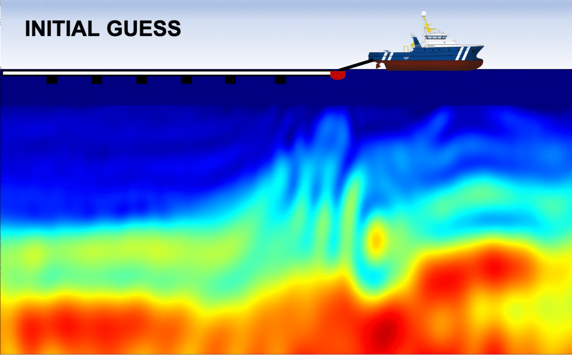
Disclaimer: the figure above (especially the boat) is not drawn to scale! The vertical extent of each panel images is approximately 3.5 km in depth by 18 km in width.
Finally, once the velocity model estimation step has been successfully conducted, it can be used (along with the seismic data) as an input to produce higher-resolution images of the subsurface. This is the last step of the imaging process, referred to as migration.