STEP 3: The migration process
In this last step, the seismic image is produced with an algorithm called migration, which is the process by which seismic recordings (seismograms) are "geometrically re-located in space to the location the event occurred in the subsurface" (according to wikipedia).
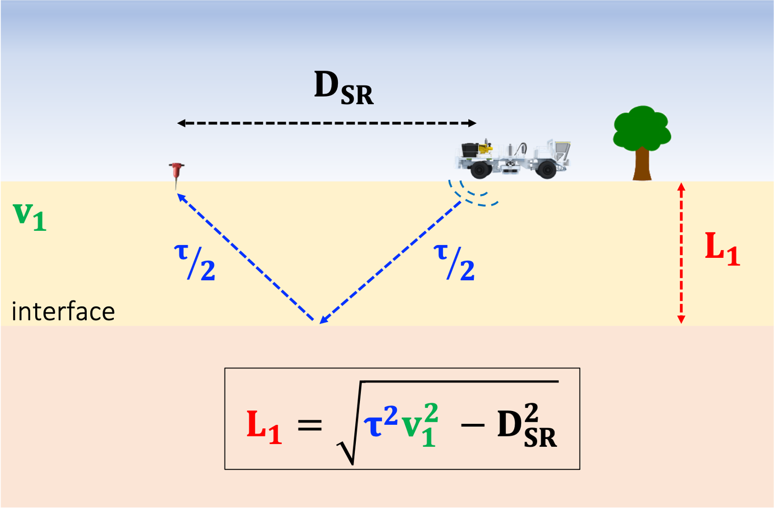
Now let's try to understand migration more intuitively on a simple case with the help of the schematic diagram shown in the figure below. A wave is sent into the ground at t0, propagates through a first layer of unknown thickness L1, reflects off an interface, and gets recorded at the surface at t1=t0+τ, where τ corresponds to the time it took for the wave to travel from the source to the interface, and from the interface to the sensor.
If the source-sensor distance DSR and the propagation speed (i.e., the velocity model) v1 in the first layer are known, it is possible (using Pythagorean theorem) to infer the position of the interface (i.e., the thickness L1 of the first layer) that gave rise to the reflection, as shown by the equation at the bottom of the figure. Indeed, for more complex geological settings, this equation does not hold, and numerical methods must be employed, such as reverse time migration (RTM).
The take-away message here is that migration is simply the process of using the reflected energy present in the recorded signal and determining the depth of the rock interface that generated this reflection.
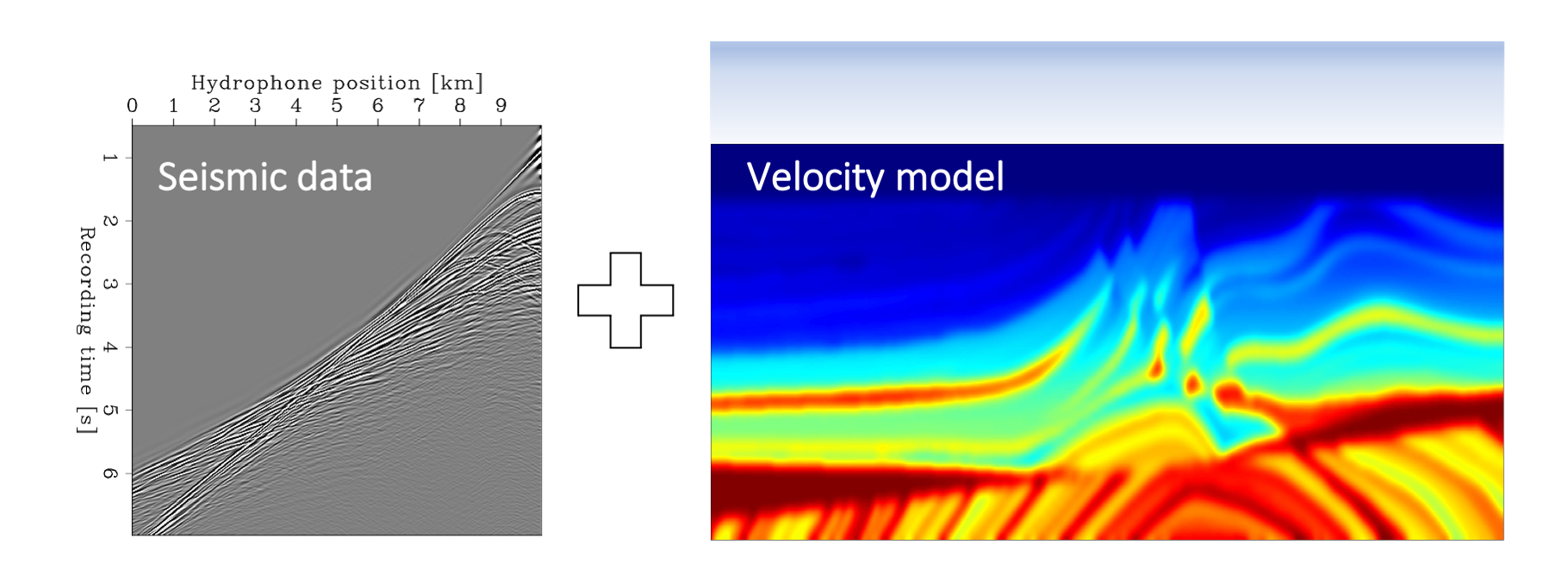
The inputs for the migration step are the seismic data acquired in the field (step 1 of the imaging process) and the seismic velocity model obtained in step 2. The figure below illustrates these inputs for the same synthetic numerical example used in the previous sections (the Marmousi 2 model). The left panel shows the seismic data as if it had been acquired with an offshore survey, and the right panel is the velocity model obtained after 100 iterations of FWI.
The output of migration is a map (referred to as a migrated image) displaying sharp boundaries between rock layers of different types (e.g., sandstone, shales, basalt, etc.). The figure below displays an example of such image. The black/white pixels indicate the presence of an interface, while the gray color corresponds to homogenous regions. The resolution of this map is higher than the one of the velocity model (right panel in the figure above) and more details about the Earth can be observed.
Finally, a team of experts will interpret the geological features of the subsurface by examininig this map (as shown by the colored annotations on the figure above), and use this additional information to infer the presence/location of hydrocarbon reservoirs. Hence, the accuracy and quality of the final migrated image will greatly impact the planning of the hydrocarbon reservoir identification, production phases, and the business-decision process.
This is where my thesis starts
In complex geological scenarios, seismic images are highly sensitive to the accuracy of the velocity model obtained by tomography, and even a small error will easily deteriorate the image quality. Unfortunately, the velocity model estimation step is extremely challenging and remains the main bottleneck of the imaging workflow. The success of conventional methods (such as FWI) is contingent on having a good initial guess, which is not always available. Therefore, a lot of research has been conducted to invent new tomography techniques robust enough to bypass the need for an accurate initial model. And this is where my thesis starts! But first, let's see why conventional methods can fail in certain scenarios