Seismic velocity estimation: the main bottleneck
As we saw in the previous sections, seismic velocity model building techniques such as FWI can be very powerful. However, it turns out that building a good velocity model can be a very difficult task. I see at least 4 main challenges for that:
1. The large number of unknown parameters
The area within the subsurface to be characterized needs to be spatially discretized into a 3D array of voxels, and then stored on a computer. The (unknown) value of each voxel represents the speed of sound at a given location, and must be numerically estimated. For field applications, the number of unknown parameters can be extremely large. For instance, a survey area with a horizontal extent of 10 km x 10 km with a maximum depth of 10 km and discretized with a spatial sampling of 10 m (which is quite commmon for industry standards) requires the estimation of as many as 109 parameters.
2. The computational cost
Tomographic algorithms require the use of iterative numerical methods based on minimizing a loss function with gradient-descent optimization schemes. At each iteration, thousands of wave propagations must be simulated on a computer, usually by numerically solving a wave-equation partial differential equation (PDE). This requirement, combined with the high-dimension nature of the problem make these algorithms very computationally intensive, even with the use of graphics processing units (GPUs).
Finally, unlike most supervised deep learning problems, the computational cost of tomographic algorithms is so high that a thorough hyperparameter search is often computationally untractable. For instance, one single forward pass of our modeling scheme could take up to 1-2 days on a modern industry-sized computer cluster. Consequently, a lot of effort is being invested into reducing the number of adjustable hyperparameters within the velocity estimation process (this is one of the main contributions of my thesis).
3. The ill-posedness of the inverse problem
The most challenging issue comes from the fact that conventional seismic tomography (using reflection data) is a mathematically and numerically ill-posed problem. In other words, the quality of the estimated solution is contingent on already having a good initial guess and/or access to a certain type of seismic data which are either too costly - or impossible - to acquire. In fact, if the initial guess is too far from the true solution, most gradient-descent optimization schemes tend to recover non geologically realistic (and thus non-useful) models. From an optimization standpoint, this phenomenon can be explained by the presence of multiple spurious local minima within the loss function that is being minimized.
4. The Earth is flat 😱
... at least for scales we are considering in hydrocarbon exploration! Unlike computed tomography (x-ray imaging), the angular covergage for seismic acquisition is more limited because it is extremely difficult (and/or costly) to place sensors deep into the ground, such as vertical seismic profiling (VSP). Hence, we are usually restricted to setting the receivers at the surface, thereby limiting our recordings to of either reflected waves or refracted energy (e.g., head waves, diving waves, etc.). For instance, such configuration may prevent us from recording energy coming from certain regions of the subsurface, thereby creating "shadow zones" where our velocity estimation is uncertain.
A numerical example where FWI fails
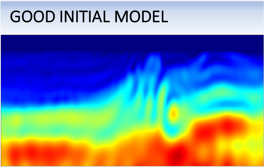
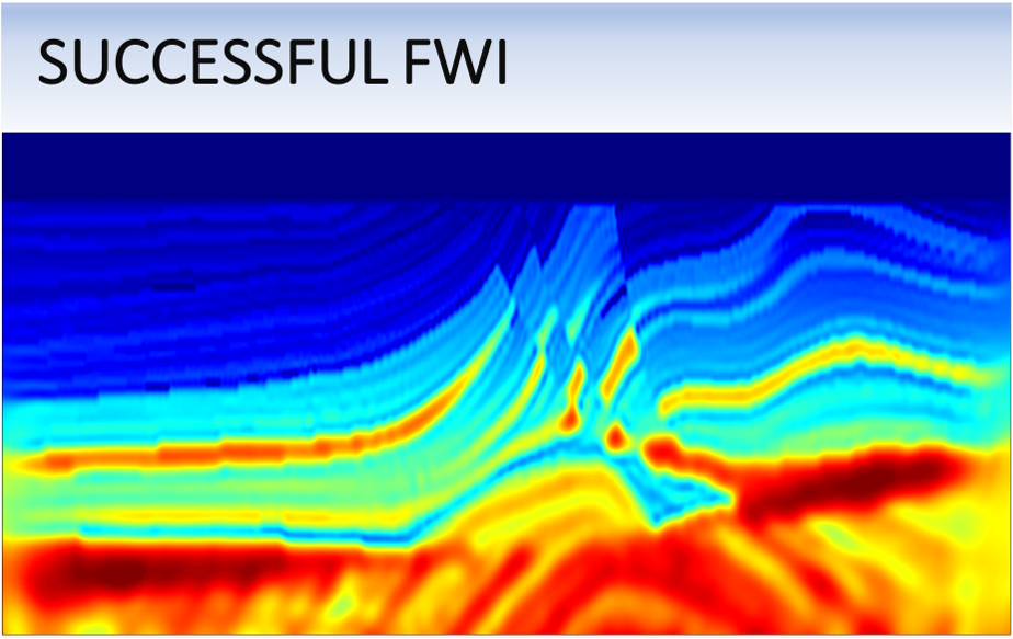
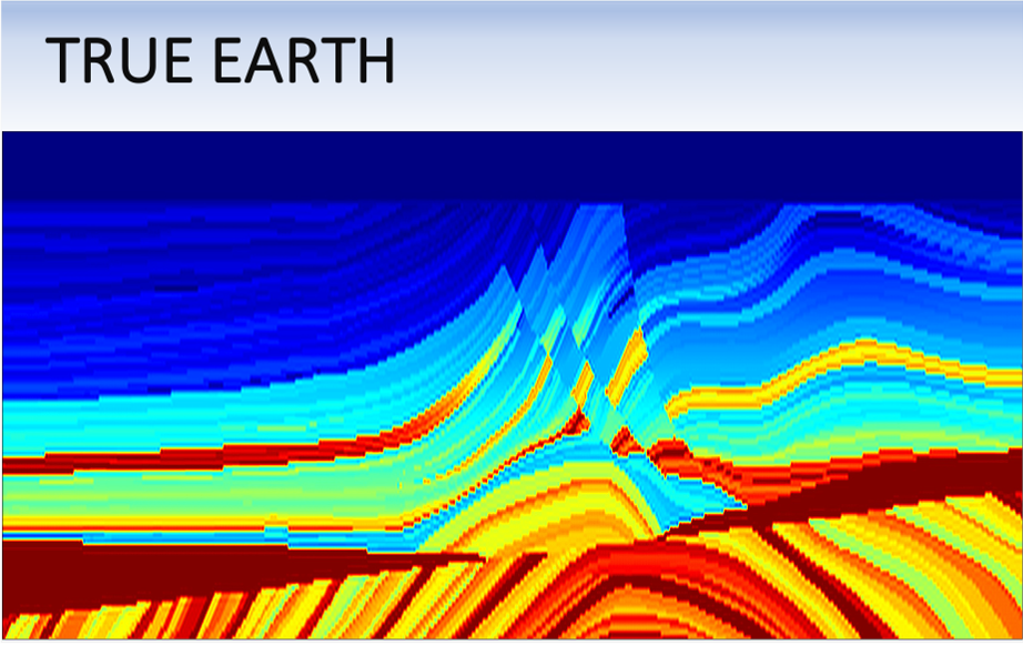
For the sack of simplicity, let's use the same benchmark model shown in the previous sections. Here I will show two cases of FWI. First, I conduct FWI starting with an accurate model, as shown in the left panel in the figure below. After 100 iterations of FWI, the recovered model (middle panel) is very accurate and similar to the true Earth (right panel). So far, so good.
We now conduct the same experiment but starting with a lower-resolution and quite uniformative initial model (left panel). As we can observe, FWI fails to recover an accurate solution (middle panel).
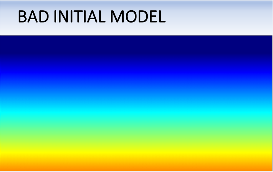
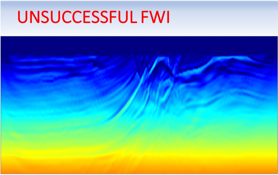
Disclaimer: all the figures above are not drawn to scale! The vertical extent of each panel is approximately 3.5 km in depth by 18 km in width.
In the next section, I show how the algorithm I developed for my Ph.D., referred to as Full Waveform Inversion by Model Extension (FWIME), mitigates this issue. Let's have a look.